Home
Examples of four elementary functions in R
![]() Loading the compressed file [folder:"ADT_R"] of source codes and data
Loading the compressed file [folder:"ADT_R"] of source codes and data
The codes of these four functions and their contexts of use are pedagogical examples of the book Analyse des Données Textuelles [Textual Data Analysis] (L. Lebart, B. Pincemin, C. Poudat), Presses de l'Université du Québec [in French], 2019.
The R software is both a language and a library. Like Python, it is a free, and cross-platform software. It is the non-proprietary component of the S programming language (Chambers, 1998), itself derived from work of a team of Bell Laboratories dating back to 1976 (team composed of Rick Becker, John Chambers, Doug Dunn, Paul Tukey, and Graham Wilkinson).
1- Compression and reconstruction of images (with graphical display)
2- Principal components analysis (with graphical display)
3- Correspondence analysis (with graphical display)
4- Computation and Plot (on a principal plane) of the Minimum Spanning Tree
![]()
1- Compression and reconstruction of images (with graphical display)
It's just about penetrating, thanks to R, into the black box of a commonplace functionality available in most statistical software of image analysis.
Evidently, the code could be much more compact, but perhaps less readable.Commands for the R interface
#-------------------------------------
source("c:\\ADT_R\\svd_image_E.r")  # source code
path= "c:\\ADT_R\\Cheetah.txt"    # data
X=read.table(path, header=FALSE, row.names=1, sep = "")
nd = 8    # number of axes for the reconstitution (e.g.)
Y = recons(X, nd)
visu_image(Y)
#-------------------------------------
The small data-test file “Cheetah.txt” is provided in the folder ADT_R. It is a simple numerical table (200 x 320) [gray levels for each pixel]. See: Nelson M. (1993). La compression des données. Text, images, sons. Dunod, Paris.
Case of a more general image in ".pgm" format (Portable Gray Map)
The "Cheetah.txt" file in the example is a simple matrix which is more rustic than the more common image formats (bmp, jpg, png).
Such images must be converted to pgm format by a free software such as GIMP or IrfanView, and the X matrix of command lines is then obtained by the four command lines below:
#-------------------------------------
# Four command lines to substitute to the line:
# "X = read.table ..." in the case of an image in pgm format
#-------------------------------------
install.packages ( "pixmap"); # to use only the first time ...
library (pixmap); # Loading the "pixmap package"
imag = read.pnm (""c:\\ADT_R\\Cheetah.pgm"); # for a "pgm" image
X = 255 * imag @ gray; # We can now call the function recons ()
#-------------------------------------
The image below is the image produced by the function recon():
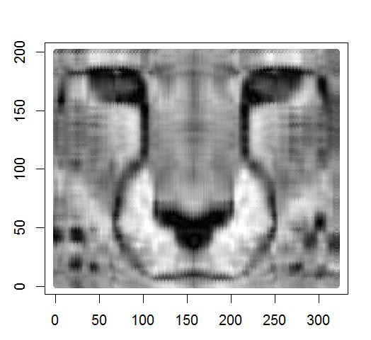
Image obtained after typing the previous R command lines. Compression rate 200/8 = 25 (8 principal axes).
![]()
A2- Principal components analysis (with graphical display)
It's just about obtaining, thanks to R, a functionality available in most statistical software of exploratory multivariate analysis.
Again, the code could be much more compact, but perhaps less readable.Commands for the R interface
#-------------------------------------
# Commands to be typed in the R interface.
source("c:/ADT_R/ACPS_E.r")             # location of source code
path= "c:/ADT_R/Mini_Semio.txt"         # location of data
X=read.table(path, header=TRUE, row.names=1, sep = ",") # X = data table
Y =ACP(X)                               # main function
plot_ind (Y, X, hor=2, ver=3, font = 1) # graph of individuals (lines)
                                         # (plane (2, 3) )
plot_var (Y, X, hor=2, ver=3, font = 1) # graph of variables (columns)
                                         # (plane (2, 3) )
#--------------------------------------------------
The small data-test file “Mini_semio.txt” is provided in the folder ADT_R. It is a simple numerical table (12 x 7) giving the scores given by 12 respondents to a set of 7 words. The real semiometric list contains 210 words, and sample sizes vary from 800 to several thousands. See:
The Semiometric Challenge: Words, Lifestyles and Values
(L. Lebart, J-F. Steiner, M. Piron, J. Wisdom), L2C, 2014.
![]() (Download the Book - pdf)
(Download the Book - pdf)
![]() (Download the book cover - pdf)
... and (in French) La sémiométrie (L. Lebart, M. Piron, J.-F. Steiner), Dunod, 2003.
(Download the book cover - pdf)
... and (in French) La sémiométrie (L. Lebart, M. Piron, J.-F. Steiner), Dunod, 2003. ![]() (Download the Book - pdf)
(Download the Book - pdf)
Small test data table ("Mini-semio.txt")
   arbre, cadeau, danger, morale, orage, politesse, sensuel
R01,  7,   4,     2,      2 ,     3 ,        1 ,     6
R02,  6 ,  3 ,    1 ,     2 ,     4 ,        1 ,     7
R03,  4 ,  5 ,    3 ,     4 ,     3 ,        4 ,     3
R04,  5 ,  5 ,    1 ,     7 ,     2 ,        7 ,     1
R05,  4 ,  5 ,    2 ,     7 ,     1 ,        6 ,     2
R06,  5 ,  7 ,    1 ,     5 ,     2 ,        6 ,     5
R07,  4 ,  2 ,    1 ,     3 ,     5 ,        3 ,     6
R08,  4 ,  1 ,    5 ,     4 ,     5 ,        4 ,     7
R09,  6 ,  6 ,    2 ,     4 ,     7 ,        5 ,     5
R10,  6 ,  6 ,    3 ,     5 ,     3 ,        6 ,     6
R11,  7 ,  7 ,    6 ,     7 ,     7 ,        6 ,     7
R12,  2 ,  2 ,    1 ,     2 ,     1 ,        3 ,     2
Meaning of the columns (words of the semiometric list):
arbre = tree; cadeau = gift;
danger = danger. morale = moral;
orage = storm; politesse = politeness;
sensuel = sensual.
The image below is the image produced by the functions ACP() and plot_ind:
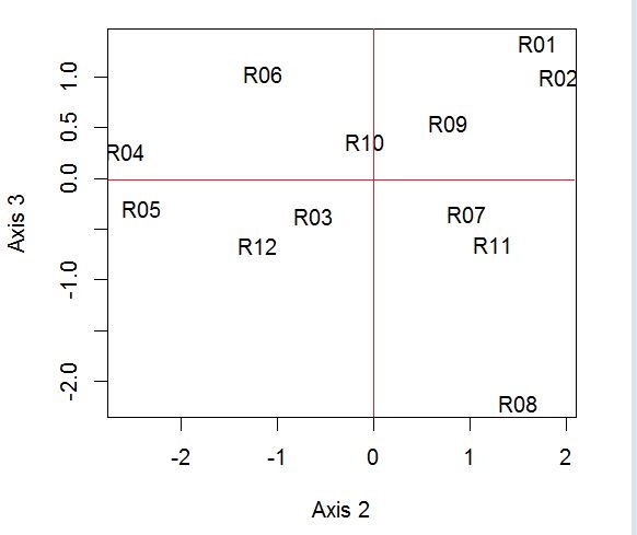
Image obtained after typing the first five R command lines.
Display of the 12 respondents in the plane (2, 3)
![]()
3- Correspondence analysis (with graphical display)
This is a simple and autonomous code for Correspondence Analysis, including a simultaneous representation of rows and columns.
Again, the code could be much more compact, but perhaps less readable.Commands for the R interface
#-------------------------------------
# Commands to be typed in the R interface.

#----------------------------------------------------------------------
# function Y = afcor(X) : Correspondence Analysis of matrix X
#----------------------------------------------------------------------
# Example for a contingency table "tab.csv" in the folder ADT_R
# (the source code:  - afcor_E.r -  being in the same folder)
 source("c:/ADT_R/afcor_E.r")          # location of source code
 path = "c:/ADT_R/tab.csv"        # location of data
# path leads to an Excel(c) file [format csv]
 X = read.csv(path, row.names = 1, sep = ";") # X = data table
 Y = afcor(X)
 plot_simult(Y) # simultaneous plot of rows and columns of the data table
#----------------------------------------------------------------------
The small data-test file “tab.csv” is provided in the folder ADT_R. It is a simple lexical table (12 x 6) giving the frequencies of 12 words (rows) in the responses of six categories of respondents. to the following question in a sample survey :
“No one can explain why, perhaps because of what they evoke, we find some words pleasant, others unpleasant.
1. As far as you are concerned personally, what are the words that you find most pleasant? (Cite as many words as possible).
2. What are the words that you find most unpleasant? (Cite as many words as possible).”
This is a case of "Open semiometry" (without closed list of words),
cf. Chapter 4 of the already quoted book: The Semiometric Challenge: Words, Lifestyles and Values
(L. Lebart, J-F. Steiner, M. Piron, J. Wisdom), L2C, 2014.
![]() (Download the Book - pdf)
(Download the Book - pdf)
![]() (Download the book cover - pdf)
... and (in French) La sémiométrie (L. Lebart, M. Piron, J.-F. Steiner), Dunod, 2003.
(Download the book cover - pdf)
... and (in French) La sémiométrie (L. Lebart, M. Piron, J.-F. Steiner), Dunod, 2003. ![]() (Download the Book - pdf)
(Download the Book - pdf)
Small test data table ("tab.csv")
Ident ; Hm30;Hm55;Hp55;Fm30;Fm55; Fp55
Translations
argent ; 11; 15; 6; 14; 9; 3 money
courage ; 2; 3; 11; 1; 3; 4 brave
dormir ; 8; 3; 1; 6; 2; 0 to sleep
livre ; 2; 7; 1; 9; 11; 11 a book
maman ; 0; 3; 0; 12; 11; 3 mother
manger ; 9; 5; 1; 10; 3; 1 to eat
pardon ; 1; 2; 6; 0; 5; 5 sorry
peinture ; 0; 0; 1; 2; 7; 3 painting
plaisir ; 10; 6; 2; 11; 2; 1 pleasure
politesse; 0; 1; 5; 0; 4; 8 politeness
repas ; 3; 5; 4; 0; 3; 1 meal
soleil ; 26; 32; 23; 54; 56; 42 sun
Meaning of the columns (categories of respondents):
Hm30 = Male, less than 30;
Hm55 = Male, between 30 and 55;
Hp55 = Male, over 55.
Fm30 = Female, less than 30;
Fm55 = Female, between 30 and 55;
Fp55 = Female, over 55.
The image below is the image produced by the functions afcor() and plot_simult():
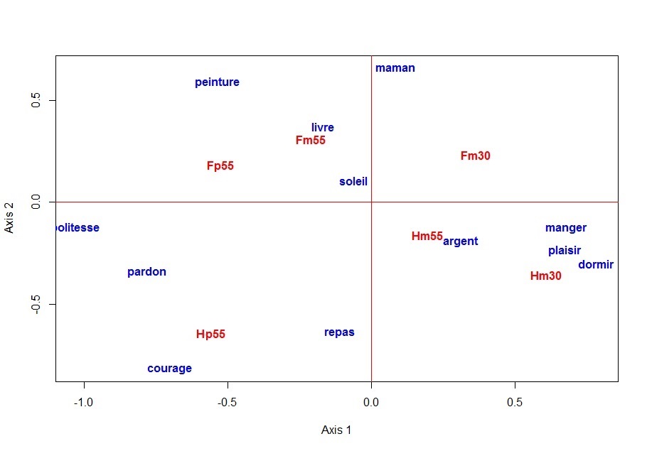
Image obtained after typing the above five R command lines.
![]()
A4- Computation and Plot(on a principal plane) of the Minimum Spanning Tree
The basic R language is used again voluntarily without any specialized library.
A choice had to be made between the many clustering methods. We chose to implement here the minimum spaning tree (armin function) using the Prim algorithm. The functions print_armin and plot_armin respectively give the list of the edges of the tree, and a representation of it in a principal plane. The tree is calculated here from the main coordinates resulting from a correspondence analysis (afcor function in section A3 above ). With these coordinates, the usual Euclidean distance corresponds to the Chi-2 distance on the initial data.
Finally, a small function afcor_armin_plot (see the end of the listings) provides the desired sequence. It is included in the file armin.r, itself included in the folder titled ADT_R.
To obtain the desired results, simply write the following lines:
Commands for the R interface
#-------------------------------------
# Commands to be typed in the R interface.

#----------------------------------------------------------------------
# composite function Y = afcor_armin_plot(X) [in the downloaded folder ADT_R]
#----------------------------------------------------------------------
# Example for a contingency table "tab.csv" in the folder ADT_R
# (the source codes: afcor_E.r and armin_R.r  being in the same folder ADR_r)
 source("c:/ADT_R/afcor_E.r")    # location of source code 1
 source("c:/ADT_R/armin_E.r"))   # location of source code 2
 path = "c:/ADT_R/tab.csv"       # location of data
# same data as in section A3
  afcor_armin_plot(path)
#----------------------------------------------------------------------
The table below is produced by the function afcor_armin_plot():
Table of vertices obtained after typing the above four R command lines.
    NumDeb   edge  NumFin     NomDeb   edge   NomFin

 [1,] 1      -----  9         argent   -----  plaisir
 [2,] 9      -----  6         plaisir  -----  manger
 [3,] 6      -----  3         manger   -----  dormir
 [4,] 1      -----  12        argent   -----  soleil
 [5,] 12     -----  4         soleil   -----  livre
 [6,] 4      -----  5         livre    -----  maman
 [7,] 1      -----  11        argent   -----  repas
 [8,] 4      -----  8         livre    -----  peinture
 [9,] 12     -----  7         soleil   -----  pardon
[10,] 7      -----  10        pardon   -----  politesse

NumDeb = Origin Number; NumFin = End Number
NomDeb = Origin Identifier; NomFin = End Identifier
The image below is the image produced by the function afcor_armin_plot():
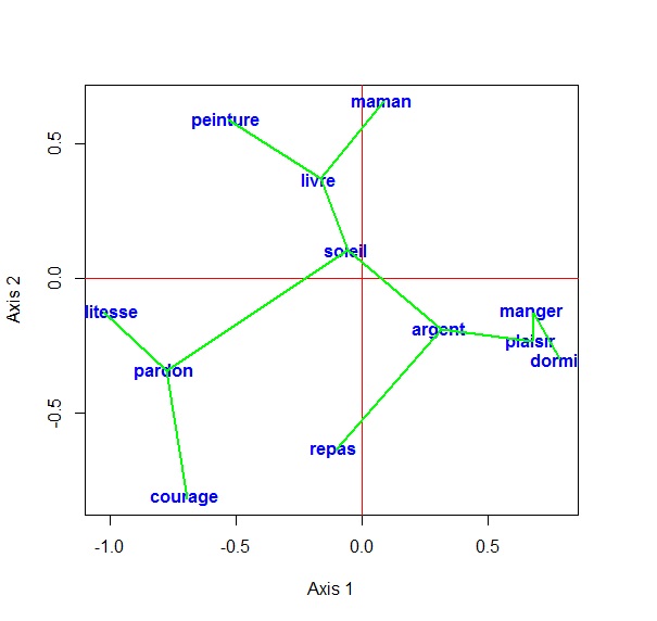
Image obtained after typing the above four R command lines.
Home